Transformer Is Inherently a Causal Learner

What if the foundation models we use every day are secretly learning the causal structure of the world? We show that transformers trained for prediction are inherently causal learners—their gradient sensitivities reveal the true cause-and-effect relationships in data, without any explicit causal training objectives.

The Big Picture

Causal discovery—figuring out what causes what—is fundamental to science. Traditional methods require specialized algorithms with strong assumptions. Meanwhile, transformers have become the backbone of modern AI, excelling at prediction tasks across domains.

Our key insight: These two worlds are deeply connected. When a transformer learns to predict the future from the past, it must implicitly learn which past variables actually matter for each prediction. This is exactly what causal discovery aims to find.

From Prediction to Causation

Consider a p-variate time series X_t = (X_1,t, …, X_p,t) and a lag window L ≥ 1. Each variable follows:

X_i,t = f_i(Pa(i,t), U_t, N_i,t)

where Pa(i,t) are the lagged parents, U_t are unobserved processes, and N_i,t are mutually independent noises.

Identifiability Assumptions

• A1. Conditional Exogeneity: Allows latent confounders as long as they don’t create spurious dependencies
• A2. No instantaneous effects: All parents occur at lags ℓ ≥ 1
• A3. Lag-window coverage: The chosen L includes all true parents
• A4. Faithfulness: The distribution is faithful to the causal graph

Theorem: Causal Identifiability via Prediction

Under A1–A4 and regularity conditions, the lagged causal graph G* is uniquely identifiable via the score gradient energy: edge j → i at lag ℓ exists if and only if H^ℓ_j,i := 𝔼[(∂_xj,t-ℓ log p(X_i,t | X_<t))²] > 0.

This theorem characterizes causal parents through sensitivity of the conditional distribution to each input. Unlike classical Granger causality which tests mean prediction, the score gradient energy captures influence on the entire conditional distribution. Gradient sensitivity = causal relevance.

Why Transformers Are Natural Causal Learners

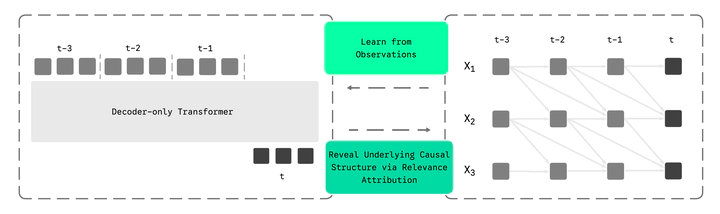
We connect the identifiability theorem to decoder-only transformers through four key properties:

1. Alignment with Identifiability: Causal masking enforces temporal precedence (A2); the window L bounds maximum lag (A3); autoregressive training naturally fits conditional distributions

2. Scalable Sparsity: Finite capacity and weight decay compress observations into generalizable parameters; softmax attention induces competitive selection among candidates; multi-head context supports selecting complementary parents

3. Contextual Parameters: Attention matrices are input-conditioned, adapting to heterogeneity and non-stationarity—different contexts induce distinct dependency patterns, enabling a mixture-of-graphs view

4. Gradient-Based Extraction: We use Layer-wise Relevance Propagation (LRP) to compute how much each past variable contributes to each prediction, then aggregate and threshold to recover the causal graph

Experimental Results

We evaluate decoder-only transformers against state-of-the-art causal discovery algorithms including PCMCI, DYNOTEARS, VAR-LiNGAM, NTS-NOTEARS, TCDF, and Granger causality tests.

Overall Performance

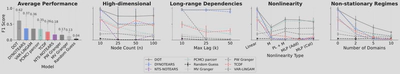
The transformer recovers lagged parents accurately and consistently across settings, achieving 0.62 average F1—nearly doubling the best baseline (DYNOTEARS at 0.37). Traditional methods degrade as dynamics and dimension grow, whereas the transformer remains robust without sensitive hyperparameter tuning.

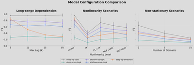
Modeling Nonlinear Interactions

We examine settings from simple to complex: linear, monotonic, piecewise linear, MLP with additive noise, and MLP with concatenated noise.

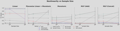
We observe a trade-off between data efficiency and expressivity. Traditional methods with simple estimators can achieve good performance efficiently in linear settings, but decoder-only transformers excel when modeling complex nonlinear dynamics and when data scales.

Scaling in Non-Stationary Settings

We construct two types of non-stationarity: (1) regular setting with randomly sampled linear structures per domain, and (2) extreme setting with random structures and nonlinear functions per domain.

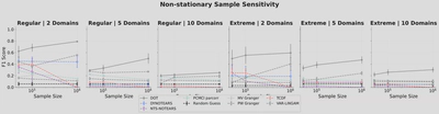
Unlike traditional methods that become intractable with more data, transformers exhibit scaling—accuracy improves consistently with sample size. The model learns to handle multiple local mechanisms within a single framework, better separating and routing different causal structures as data increases.

Robustness to Noise and Latent Variables

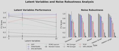
Transformers demonstrate robust performance across different noise distributions, maintaining consistent accuracy regardless of noise type or variance properties. However, due to the lack of a latent variable modeling mechanism, transformers can learn spurious links when latent confounders are present.

Handling Real-World Complications

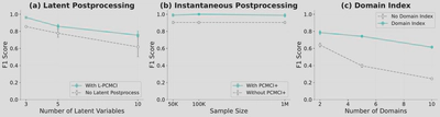
Latent Confounders: We show that post-processing with latent-aware methods like L-PCMCI, starting from transformer-predicted edges, sharply reduces the search space and yields substantially higher accuracy.

Instantaneous Relationships: By combining the learned structure with algorithms that handle contemporaneous relationships (e.g., PCMCI+), we can refine confounded graphs and recognize instantaneous effects.

Domain Indicators: Encoding domain indices as additional input helps the transformer separate cross-domain changes from invariants, improving data efficiency in non-stationary settings.

Attention vs. Gradient Attribution

We find that raw attention scores work better in shallow (1-layer) transformers but fail in deeper models. As depth increases, repeated attention routing and residual MLP updates mix token representations, making attention unreliable for structure recovery. LRP-based gradient attribution consistently outperforms attention-based methods, especially in deep transformers suited for complex dynamics.

Uncertainty Analysis

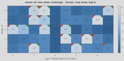
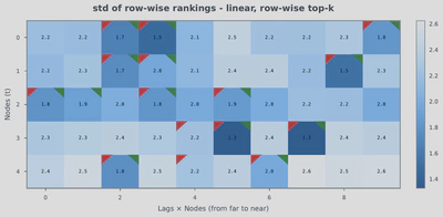
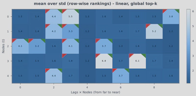
Statistical causal discovery estimates uncertainty via resampling. With transformers, we aggregate per-sample estimates and use their standard deviation to gauge consistency. True edges show higher mean rankings and lower variance, offering a pragmatic way to surface reliable edges when precision is prioritized.

Additional Analysis

Intervention Effects Align with Gradient Attributions

To validate that gradient-based attributions truly capture causal relationships, we compare them with intervention-based effects (the gold standard in causal inference). We intervene on input variables by one standard deviation and measure the average effect on outputs.

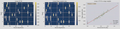
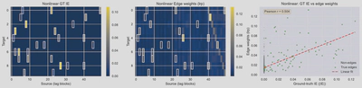
The strong correlation between intervention effects and gradient attributions confirms that the transformer’s internal representation genuinely captures causal structure, not just statistical associations.

Can Current Foundation Models Discover Structure Zero-Shot?

We explore whether existing time-series foundation models (Chronos2) can perform zero-shot causal discovery.

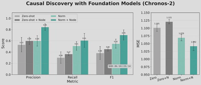
Key findings:

• Zero-shot forecasting accuracy is reasonable but structure recovery is suboptimal
• Raw time-series data is less structured and noisier than language, making it hard to learn generalizable inductive biases
• Even with large-scale pretraining, effective sample size for learning dynamics is insufficient
• Finetuning on domain-specific data significantly improves both forecasting and causal discovery
• Adding node embeddings (even randomly initialized) helps the model distinguish variables and improves structure recovery

Current time-series foundation models can serve as noisy zero-shot discoverers but may require domain adaptation for practical applications.

Realistic Non-Stationary Settings with Minimal Changes

Real-world systems often exhibit gradual, minimal changes across regimes rather than completely random structure shifts.

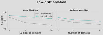
When regime changes are minimal and gradual (more realistic), data efficiency is substantially higher compared to randomly sampled settings. This demonstrates the practical applicability of our approach to real-world scenarios where causal structures evolve slowly over time.

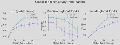
Sensitivity Analysis: Graph Binarization

The choice of top-k in graph binarization affects the precision-recall trade-off.

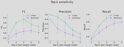
Recommendations:

• Use row-wise top-k when variables have similar numbers of parents
• Use global top-k when parent counts vary across variables
• Visualize the heatmap of edge scores for flexible threshold selection based on task requirements (precision vs. recall)

Implications

For Causal Discovery

This work opens a new paradigm: instead of hand-crafting discovery algorithms, we can leverage the representation learning capabilities of foundation models. The transformer becomes a universal causal structure extractor that scales with data.

For Foundation Models

The causal perspective offers new tools to understand and improve large models:

• Interpretability: Gradient attributions reveal learned dependencies
• Hallucinations: May arise when insufficient data prevents accurate structure learning—the model resorts to spurious correlations when it cannot adequately separate regimes
• Architecture design: Causal priors (sparsity, modularity) could guide better architectures

Citation

@inproceedings{wang2025transformer,
  title={Transformer Is Inherently a Causal Learner},
  author={Wang, Xinyue and Wang, Stephen and Huang, Biwei},
  booktitle={NeurIPS 2025 Workshop on CauScien},
  year={2025}
}